Boundary Conditions
Contents
Boundary Conditions#
In [1]: import xarray as xr

In [2]: import numpy as np

In [3]: from xgcm import Grid

In [4]: ds = xr.Dataset(
   ...:     coords={
   ...:         "x_c": (
   ...:             ["x_c"],
   ...:             np.arange(1, 10),
   ...:             {"axis": "X"},
   ...:         ),
   ...:         "x_g": (
   ...:             ["x_g"],
   ...:             np.arange(0.5, 9),
   ...:             {"axis": "X", "c_grid_axis_shift": -0.5},
   ...:         ),
   ...:     }
   ...: )
   ...:

In [5]: ds
Out[5]:
<xarray.Dataset>
Dimensions:  (x_c: 9, x_g: 9)
Coordinates:
  * x_c      (x_c) int64 1 2 3 4 5 6 7 8 9
  * x_g      (x_g) float64 0.5 1.5 2.5 3.5 4.5 5.5 6.5 7.5 8.5
Data variables:
    *empty*
Boundary condition choices#
For variables located at the boundaries, some operations need boundary conditions. Let’s use the previous example axis, with center and left points:
|     |     |     |     |
U--T--U--T--U--T--U--T--|
|     |     |     |     |
If we have a variable at the U (left) points, we have a problem for some operation (e.g. differentiating): how to treat the last T point? The solution is to add an extra point for the computation (‘X’ point on the following sketch):
|     |     |     |     |
U--T--U--T--U--T--U--T--X
|     |     |     |     |
Different options are possible (fill this extra value with a certain number,
extend to the nearest value, or periodic condition if the grid axis is periodic).
Note that this boundary condition is used to give the value of X, not to give the value of the
boundary T point after the operation.
We can illustrate it by creating some data located at the U point:
In [6]: g = np.sqrt(ds.x_g + 0.5) + np.sin((ds.x_g - 0.5) * 2 * np.pi / 8)

In [7]: g
Out[7]:
<xarray.DataArray 'x_g' (x_g: 9)>
array([1.        , 2.12132034, 2.73205081, 2.70710678, 2.23606798,
       1.74238296, 1.64575131, 2.12132034, 3.        ])
Coordinates:
  * x_g      (x_g) float64 0.5 1.5 2.5 3.5 4.5 5.5 6.5 7.5 8.5
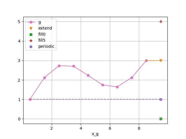
We show here the value of the extra added point for 5 cases (extended, filled with 0, filled with 5,
and periodic). The periodic condition is not an argument of the methods, but is provided
as an argument of the xgcm.Grid. We will thus also create 2 grids: one periodic and another one not periodic.
In [8]: def plot_bc(ds):
   ...:     plt.plot(ds.x_g, g, marker="o", color="C6", label="g")
   ...:     #
   ...:     plt.scatter([ds.x_g[-1] + 1], [g[-1]], color="C1", label="extend", marker="v")
   ...:     plt.plot(
   ...:         [ds.x_g[-1], ds.x_g[-1] + 1], [g[-1], g[-1]], "--", color="C1", label="_"
   ...:     )
   ...:     #
   ...:     plt.scatter([ds.x_g[-1] + 1], [0], color="C2", label="fill0", marker="s")
   ...:     plt.scatter([ds.x_g[-1] + 1], [5], color="C3", label="fill5", marker="P")
   ...:     #
   ...:     plt.scatter([ds.x_g[-1] + 1], g[0], color="C4", label="periodic", marker="X")
   ...:     plt.plot([ds.x_g[0], ds.x_g[-1] + 1], [g[0], g[0]], "--", color="C4", label="_")
   ...:     #
   ...:     plt.xlabel("x_g")
   ...:     plt.legend()
   ...:     return
   ...:

In [9]: plot_bc(ds)
If we now compute the difference using the 5 conditions:
In [10]: grid_no_perio = Grid(ds, periodic=False)

In [11]: grid_perio = Grid(ds, periodic=True)

In [12]: g_extend = grid_no_perio.diff(g, "X", boundary="extend").rename("extend")

In [13]: g_fill_0 = grid_no_perio.diff(g, "X", boundary="fill", fill_value=0).rename("fill0")

In [14]: g_fill_2 = grid_no_perio.diff(g, "X", boundary="fill", fill_value=5).rename("fill5")

In [15]: g_perio = grid_perio.diff(g, "X").rename("periodic")
In [16]: for (i, var) in enumerate([g_extend, g_fill_0, g_fill_2, g_perio]):
   ....:     var.plot.line(marker="o", label=var.name)
   ....:

In [17]: plt.legend()
Out[17]: <matplotlib.legend.Legend at 0x7f102b4bfe20>
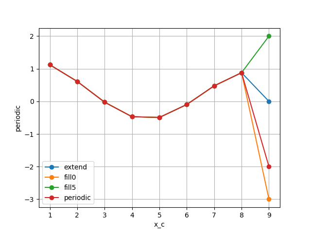
As expected the difference at x_c=9 is 0 for the case extend,
is -2 = 1 - 3 for the periodic case,
is -3 = 0 - 3 for the fill with 0 case,
and is 2 = 5 - 3 for the fill with 5 case.